I knew I wanted to build rockets at age seven, when I assembled a LEGO Saturn V rocket.
Now I'm designing an amateur N₂O/ethanol liquid bipropellant rocket from scratch —
running NASA CEA, isentropic flow equations, and Barrowman analysis to get it off the ground.
102.5"Rocket Length
235.5sTheoretical Isp
~800ftCOSMOS Apogee
J-classMotor Class
COSMOS UCLA · Summer 2025
Solid-Motor Rocket Build
In Cluster 5 at UCLA under Professor Spearrin, I learned the fundamentals of
aerospace engineering — then applied them in two weeks of hands-on manufacturing
with a small team.
Derived Tsiolkovsky rocket equation, Bernoulli's principle, isentropic flow equations, and beam bending from first principles
Designed fins in OnShape CAD; manufactured using laser cutting, waterjet cutting, and 3D printing
Assembled body tube using carbon fiber and epoxy composite — learned composite properties from the Rule of Mixtures
Validated center of pressure in wind tunnel; iterated until stability margin was sufficient
Balsa wood fins snapped under force — redesigned thicker fins with a 3D-printed alignment jig across several iterations
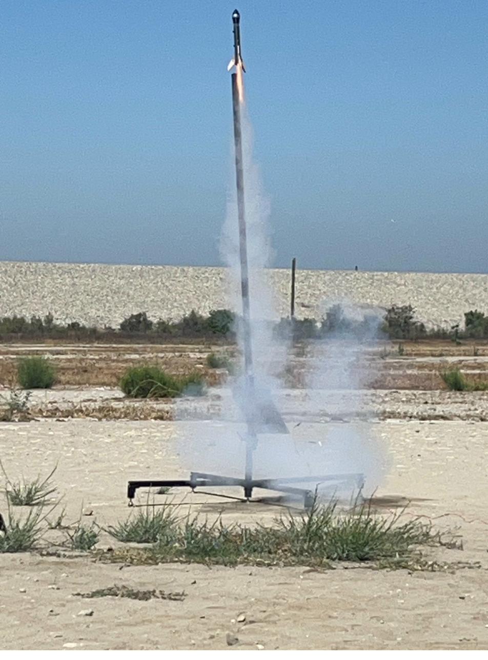
Reached approximately 800 ft apogee on a D-class motor — a successful first flight
Iteration is as fundamental as the physics.
Independent Project · In Development
Amateur Liquid Bipropellant Rocket
After COSMOS, I designed my own N₂O/ethanol liquid bipropellant rocket from scratch.
The seven-year-old with the LEGO Saturn V is still in there — he just has better tools now.
Diameter4.000 in.
Length102.5 in.
OxidizerNitrous Oxide (N₂O)
FuelEthanol (E85)
Dry Mass35.5 lbs
Motor ClassJ-class (~1220 N·s)
Combustion Temp2084 K
Injector TypeScrintle Injector
Interactive CAD Model
Full rocket assembly - designed and modeled in OnShape.
drag to rotatescroll to zoomright-click to pan
Fetching rocket assembly…
Could not load STL file. Make sure rocket.stl is in the assets/ folder.
Front
Back
Left
Right
Top
Bottom
Analysis
Isentropic Flow & NASA CEA
I used Chemical Equilibrium Analysis (CEA) to compute combustion properties, then
applied isentropic flow equations to determine nozzle geometry. These simplified
models work well — but can't capture complex shock structures in overexpanded flow,
which is why CFD is the next step.
nasa_cea_output.txtNASA CEA · N₂O / E85
# Chemical Equilibrium Analysis# Oxidizer: N2O · Fuel: Ethanol (E85)# Pc = 300 psi · MR = 3.2 · ε = 4.0
Isp (vac) = 235.5 s
C* = 1399 m/s
Tc = 2084 K
gamma = 1.21
throat area = 0.785 in²
# Derived from C* = p_c * A_t / m_dot# At gives ~270 lbf thrust at Pc = 300 psi
cea_analysis.pyPython
from rocketcea.cea_obj_w_units import CEA_Obj
cea = CEA_Obj(
oxName='N2O',
fuelName='Ethanol',
pressure_units='bar',
temperature_units='K',
isp_units='sec',
cstar_units='m/s'
)
Pc = 20.7# bar (~300 psi)
MR = 3.2# mixture ratio
eps = 4.0# expansion ratio
isp_vac = cea.get_Isp(Pc=Pc, MR=MR, eps=eps)
c_star = cea.get_Cstar(Pc=Pc, MR=MR)
Tc = cea.get_Tcomb(Pc=Pc, MR=MR)
print(f"Isp: {isp_vac:.1f} s")
print(f"C*: {c_star:.0f} m/s")
print(f"Tc: {Tc:.0f} K")
Thrust Curve — J-class (~1220 N·s)
Approximate profile · ~270 lbf average · 6s burn
Throat Area0.785 in²
Exit Velocity~2200 m/s
Total Impulse~1220 N·s
Burn Duration6 seconds
Stability Analysis
CG, CP, and Stability Margin
Using the Barrowman equations, I estimated the center of pressure from the rocket's
geometry. The stability margin of 1.55 calibers confirms
stable flight — the CP sits far enough behind the CG that aerodynamic forces will
self-correct any perturbation in trajectory.
← Nose ConeFins →
CG · 55.9"
CP · 66.2"
Stability margin: 1.55 cal· Stable · SM = (X_cp − X_cg) / D
barrowman.txtBarrowman Equations — CP Estimate
// Nose cone normal force coefficient
CN_n = 2

// Fin correction (4 trapezoidal fins)
CN_f = 4 * (1 + r/(s+r)) * (S_f / A_ref) / (1 + √(1 + (2*λ/c_m)²))

// Weighted center of pressure
X_cp = (CN_n * X_n + CN_f * X_f) / (CN_n + CN_f)

// Result
X_cp ≈ 66.2 in. from nose cone
SM   = (X_cp - X_cg) / D = (66.2 - 55.9) / 4.0 = 1.55 cal ✓
→
Next: Computational Fluid Dynamics
Simplified isentropic models have fundamental limitations — they can't capture complex
shock structures in overexpanded flow conditions. My next step is researching how
reduced-order models (ROMs) built from proper orthogonal decomposition can preserve
the key physical features of shock boundary-layer interactions in compressible flow,
bridging the gap between expensive high-fidelity CFD and the simplified models I've
been using.